A Beginner’s Guide to the MTCOV Algorithm in the probinet Package#
In this tutorial, we demonstrate how to use the Probabilistic Generative Models (probinet) package to
run the MTCOV algorithm on a sample dataset.
The MTCOV (Multitensor and Covariates) algorithm is a
probabilistic generative model designed to perform community detection and broader inference in
attributed multilayer networks, which are networks enriched with node and edge metadata [CPDB20].
Package Structure#
Before explaining how to use the MTCOV algorithm, let’s explore the structure of the probinet package, which is organized into several main modules.
1. Input#
The input module handles data input for subsequent use by the algorithms in the model module. It comprises the following submodules:
loader: Functions to load data from input files.preprocessing: Functions for data preprocessing, such as converting NetworkX graphs to sparse adjacency matrices.stats: Functions for computing statistics on the data.
2. Models#
The models module contains the implementation of various algorithms, including the following
submodules:
crep: Implementation of theCRepalgorithm.jointcrep: Implementation of theJointCRepalgorithm.dyncrep: Implementation of theDynCRepalgorithm.mtcov: Implementation of theMTCOValgorithm.acd: Implementation of theACDalgorithm.base: Base classes and utilities for the models.constants: Constants used across the models.classes: Classes used across the models.
3. Evaluation#
The evaluation module contains functions responsible for handling the outputs of the models. It
consists of the following submodules:
community_detection: Functions to evaluate the performance of community detection algorithms.expectation_computation: Functions for computing expectations and related metrics.likelihood: Functions for computing the likelihood of the model given the data.link_prediction: Functions for evaluating link prediction tasks.covariate_prediction: Functions for evaluating node covariate prediction tasks.
4. Synthetic#
The synthetic module contains functions to generate synthetic data. It consists of the following submodules:
base: Create a synthetic, directed, and weighted network (possibly multilayer) by a standard mixed-membership stochastic block-model.reciprocity: Generate directed networks with communities and reciprocity.dynamic: Create directed networks with communities and reciprocity that change over time.anomaly: Generate networks with node communities and anomalous edges.multilayer: Create attributed multilayer networks with communities.
An example of how to use the reciprocity submodule is shown in the tutorial on CRep algorithm.
5. Model Selection#
The model_selection module contains functions for model selection and cross-validation. It consists of the following submodules:
parameter_search: Functions for searching model parameters.cross_validation: Functions for performing cross-validation.mtcov_cross_validation: Cross-validation specific to theMTCOValgorithm.dyncrep_cross_validation: Cross-validation specific to theDynCRepalgorithm.acd_cross_validation: Cross-validation specific to theACDalgorithm.crep_cross_validation: Cross-validation specific to theCRepalgorithm.jointcrep_cross_validation: Cross-validation specific to theJointCRepalgorithm.masking: Functions for masking data during cross-validation.main: Main entry points for running model selection.
6. Utils#
The utils module contains utility functions used across the package. It consists of the following submodules:
matrix_operations: Functions for matrix operations.tools: General utility functions.
7. Main#
The main module contains the main entry points for running the algorithms.
8. Data#
The data module contains the data files used by the package. It consists of the following submodules:
input: Input data files.model: Configuration files for the models.
9. Visualization#
The visualization module contains functions for visualizing the results of the models. It
consists of the following submodule:
plot: the main module used for plotting.
Having explored the package structure, let’s see how to use it to run the MTCOV algorithm.
Configuration#
Let’s start by configuring the algorithm and the parameters needed. The pipeline works based on two types of parameters:
Numerical Parameters: These are operational parameters that control the execution of the algorithm. They are not directly related to the model’s theoretical framework but are crucial for its practical implementation. Examples include:
Convergence tolerance (
convergence_tol): This is a threshold used to determine when the algorithm has converged, i.e., when the changes in the model’s likelihood or parameters between iterations are small enough to consider the model as having reached its final state.Maximum number of iterations (
max_iter): This is the maximum number of times the algorithm will update the model’s parameters. If the model hasn’t converged by this point, the algorithm will stop anyway.Number of realizations (
num_realizations): This refers to the number of times the entire process (initialization and iterative updates) is repeated. The algorithm will then return the best realization, that is, for instance, the one with the highest likelihood upon convergence. This is done to account for the randomness in the initialization step and to ensure a more robust final model.
These are set by default in the model’s class definition, but they can be changed by the user.
Model parameters: These are parameters that are part of the model’s theoretical framework. They have a direct impact on the model’s behavior and the results it produces. Examples include:
Number of communities (
K): This is a fundamental parameter of the algorithms presented in this package. It determines the number of communities the algorithm will try to find in the network.Scaling parameter (
gamma): This is a fundamental parameter of theMTCOValgorithm. It controls the relative contribution of the two terms in the likelihood, which accounts for network topology and node covariates, respectively. Whengamma=0, the inference is performed by analyzing the data purely in terms of the network topology. Vice versa, whengamma=1, the algorithm only uses the attribute information.
Notice that the data is not a parameter, but an input to the algorithm, hence, it is not included in the default configuration of the class nor in the configuration file. This will be shown later in the tutorial.
Setting the Logger#
As a first step, let’s configure the logger to show the information about the execution of the algorithm.
# Import the logging module
import logging

# Get the root logger and set its level to INFO
logging.getLogger().setLevel(logging.INFO)
Importing the data#
We can now import the data using the probinet package.
from pathlib import Path
from probinet.input.loader import build_adjacency_and_design_from_file
from probinet.models.classes import GraphData

# Define the names of the columns in the input file that
# represent the source and target nodes of each edge.
ego = "source"
alter = "target"
egoX = "Name"

# Set the `force_dense` flag to False
# This flag determines whether the adjacency matrices
# should be stored as dense matrices.
# If set to False, the adjacency matrices will be stored
# as sparse matrices, which is more memory-efficient
# for large networks with few edges.
force_dense = False

# Get the absolute path of the root directory of the project
root_dir = Path.cwd().parent.parent.parent.resolve()

# Define the path to the input folder
in_folder = str(root_dir / "probinet/data/input/")

# Define the name of the network file
adj_name = "synthetic_multilayer_network.csv"

# Define the name of the covariates file
cov_name = "synthetic_design_matrix.csv"

# Define the attribute name
attr_name = "Metadata"

# Flag to treat the network as undirected
undirected = False

# Flag to treat the network as binary
binary = True

# Flag to remove the self-loops
noselfloop = True

# Call the `build_adjacency_and_design_from_file` function to load the data from the input file
# The function takes several arguments:
# - in_folder: the path to the data
# - adj_name: the name of the file with the adjacency matrix
# - cov_name: the name of the file with the design matrix
# - ego: the name of the column that references the node in one extreme of the directed edge
# - alter: the name of the column that references the other node
# - egoX: the name of the column to consider as node ID in the design matrix
# - attr_name: name of the attribute to consider in the analysis
# - undirected: the flag that signals if the network is undirected
# - binary: if set to True, the network is treated as binary
# - force_dense: if set to True, the network is saved in a dense adjacency tensor
# - noselfloop : if set to True, the self-loops are removed
gdata: GraphData = build_adjacency_and_design_from_file(
    in_folder,
    adj_name=adj_name,
    cov_name=cov_name,
    ego=ego,
    alter=alter,
    egoX=egoX,
    attr_name=attr_name,
    undirected=undirected,
    binary=binary,
    force_dense=force_dense,
    noselfloop=noselfloop,
)
To get some information about the data, we can call the print_graph_stats function from the
input.stats module.
from probinet.input.stats import print_graph_stats

# Extract the graph list from the `GraphData` object
A = gdata.graph_list

# Call the `print_graph_stats` function to print the basic
# statistics of the graphs in the list `A`.
print_graph_stats(A)
Number of nodes = 300
Number of layers = 4
Number of edges and average degree in each layer:
E[0] = 1294 / <k> = 8.63
Sparsity [0] = 0.014
Reciprocity (networkX) = 0.028
E[1] = 1340 / <k> = 8.93
Sparsity [1] = 0.015
Reciprocity (networkX) = 0.021
E[2] = 724 / <k> = 4.83
Sparsity [2] = 0.008
Reciprocity (networkX) = 0.030
E[3] = 742 / <k> = 4.95
Sparsity [3] = 0.008
Reciprocity (networkX) = 0.003
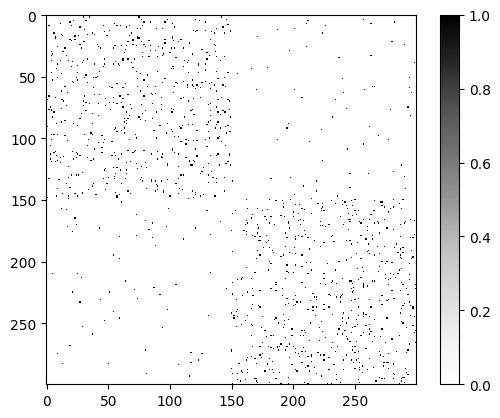
Let’s now show the adjacency matrix of one of the four layers.
import networkx as nx

# Save the graph corresponding to the first layer
graph = A[0]

# Get the adjacency matrix
adjacency_matrix = nx.adjacency_matrix(graph)
# Import the `pyplot` module from `matplotlib` for creating
# static, animated, and interactive visualizations in Python.
import matplotlib.pyplot as plt

# Display the reshaped adjacency matrix as an image
# The `imshow` function from the `pyplot` module is used to
# display data as an image.
# The `cmap` argument specifies the colormap to use for the image
# The `interpolation` argument specifies the interpolation method
# to use when resizing the image.
plt.imshow(adjacency_matrix.toarray(), cmap="Greys", interpolation="none")

# Add a color bar to the plot for reference
# The colors in the color bar correspond to the values in the image:
# black for 1, meaning a connection, and white for 0, meaning no connection.
plt.colorbar()
plt.show()

As we can see in the matrix, the network is not fully connected, i.e., there are nodes that are not
connected to any other node. This is a common characteristic of real-world networks. More
importantly, we can see that the network has two main clusters of nodes, which are represented by the two regions more densely connected. These are the communities that the MTCOV algorithm will try to detect.
Running the Model#
Finally, we are ready to run the MTCOV model! The way this works is in a two-step process:
Initialize the
MTCOVmodel by creating an instance of theMTCOVclass.Execute the
fitmethod on the created instance to run the algorithm.
# Import the `MTCOV` class from the `probinet.models.mtcov` module
# This class is used to create an instance of the `MTCOV` algorithm
from probinet.models.mtcov import MTCOV

# Create an instance of the `MTCOV` class
# The `MTCOV` class takes no arguments, unless the user wants
# to change the default of the numerical parameters.
model = MTCOV()

# Print all the attributes of the `MTCOV` instance
# The `__dict__` attribute of an object is a dictionary containing
# the object's attributes.
# These correspond to the numerical parameters
print(model.__dict__)
{'inf': 10000000000.0, 'err_max': 1e-07, 'err': 0.1, 'num_realizations': 1, 'convergence_tol': 0.0001, 'decision': 10, 'max_iter': 500, 'plot_loglik': False, 'flag_conv': 'log', '__doc__': None, 'attributes_to_save_names': ['u_f', 'v_f', 'w_f', 'eta_f', 'final_it', 'maxL', 'maxPSL', 'beta_f', 'nodes', 'pibr', 'mupr'], 'u_f': array([], dtype=float64), 'v_f': array([], dtype=float64), 'w_f': array([], dtype=float64), 'use_unit_uniform': False, 'theta': {}, 'normalize_rows': False, 'nodes': [], 'rng': Generator(PCG64) at 0x7FAC1947D9A0, 'beta_hat': array([], dtype=float64), 'best_r': 0, 'final_it': 0, 'message_for_invalid_initialization': 'The initialization parameter can be either 0 or 1. If 0, the model will be initialized randomly. If 1, the model will be initialized with the parameters stored in the file specified in the `files` parameter.'}
Model created! Now, we can run the model using the fit method. As mentioned before, this method
takes as input the data, and model parameters.
# Import the `time` module
import time

# Import the `numpy` module
import numpy as np

# Define the output folder
out_folder = "tutorial_outputs/MTCOV/"

# Fix the rng for reproducibility
rseed = 1
rng = np.random.default_rng(rseed)

# Get the current time
time_start = time.time()

# Run the `MTCOV` model
# The `fit` method of the `MTCOV` class takes several arguments:
# - gdata: the data to be analyzed
# - out_inference: if set to True, the algorithm saves the final state of the models
# - out_folder: the folder where the output files will be saved
# - end_file: the ending of the file name

_ = model.fit(
    gdata,
    out_inference=True,
    out_folder=out_folder,
    end_file="_MTCOV",
    rng=rng
)

# Print the time elapsed since the start of the `MTCOV` algorithm
print(f"\nTime elapsed: {np.round(time.time() - time_start, 2)} seconds.")
INFO:root:gamma = 0.5
INFO:root:Algorithm successfully converged after 341 iterations with a maximum log-likelihood of -10093.8593.
INFO:root:Inferred parameters saved in: /home/runner/work/probinet/probinet/docs/source/tutorials/tutorial_outputs/MTCOV/theta_MTCOV.npz
INFO:root:To load: theta=np.load(filename), then e.g. theta["u"]
Time elapsed: 1.06 seconds.
Done! The final state of the model is not returned, but it is saved to the output folder.
Analyzing the results#
Next, we will examine the outcomes produced by the model. To do this, it is necessary to load the
contents from the file theta_MTCOV.npz, generated by the fit method.
# Define the path to the file containing the results of the `MTCOV` models
filename = out_folder + "/theta_MTCOV.npz"

# Load the contents of the file into a dictionary
theta = np.load(filename)
Once this is done, we can unpack the latent variables.
# Unpack the latent variables from the results of the `MTCOV` models
# The `u` variable represents the out-going memberships of the
# nodes in the graph.
# The `v` variable represents the in-coming memberships of the
# nodes in the graph.
# The `w` variable represents the affinity of the communities
# for each layer.
# The `beta` variable represents the relationships between
# communities and covariates.
u, v, w, beta = theta["u"], theta["v"], theta["w"], theta["beta"]
As outlined in the main reference [CPDB20], MTCOV assumes a mixed-membership community structure, which
means that
every node can belong to more than one community with a different strength. The variables u and
v are NxK membership matrices that represent the out-going and in-coming node memberships,
respectively. In this specific demonstration, it’s important to recall that we configured the
model parameter K, representing the number of communities, to be 2. Consequently, by examining the values of u for each node, we expect to obtain vector of length two, where the first entry is the probability of node i to belong to community 1 and the second one represents the probability to belong to community 2.
# Iterate over the first 10 nodes in the graph
for idx, values in enumerate(u[:10]):
    # Print the probability that the node belongs to the two communities
    print(
        f"The probability that the node {idx} belongs to the two communities is: {values}"
    )
The probability that the node 0 belongs to the two communities is: [1. 0.]
The probability that the node 1 belongs to the two communities is: [1. 0.]
The probability that the node 2 belongs to the two communities is: [1. 0.]
The probability that the node 3 belongs to the two communities is: [1. 0.]
The probability that the node 4 belongs to the two communities is: [1. 0.]
The probability that the node 5 belongs to the two communities is: [0.93565105 0.06434895]
The probability that the node 6 belongs to the two communities is: [1. 0.]
The probability that the node 7 belongs to the two communities is: [1. 0.]
The probability that the node 8 belongs to the two communities is: [1. 0.]
The probability that the node 9 belongs to the two communities is: [1. 0.]
To visualize the hard-memberships for the out-going case, we can assign each node to the
community with the highest probability in u. We can then print the community assignments for the first 10 nodes.
# Calculate the hard-memberships for the out-going case
u_hard = np.argmax(u, axis=1)

# Get the indices of nodes in community 1 and community 2
community1_nodes = np.where(u_hard == 0)[0]  # Community 1 corresponds to index 0
community2_nodes = np.where(u_hard == 1)[0]  # Community 2 corresponds to index 1

# Print some nodes from community 1
print("Some nodes in community 1:")
print(community1_nodes[:10])

# Print some nodes from community 2
print("\nSome nodes in community 2:")
print(community2_nodes[0:10])
Some nodes in community 1:
[0 1 2 3 4 5 6 7 8 9]

Some nodes in community 2:
[150 151 152 153 154 155 156 157 158 159]
We have learned this way to assign each node to a community, using the results given by the
MTCOV algorithm. For a more graphical approach, we invite the reader to take a look at the tutorial on the
JointCRep algorithm, where we show how to plot the communities in the
network.
In addition to investigate the node memberships, we can interpret the relationships between the
inferred communities and the node covariate through the variable beta. As outlined in the main
reference,
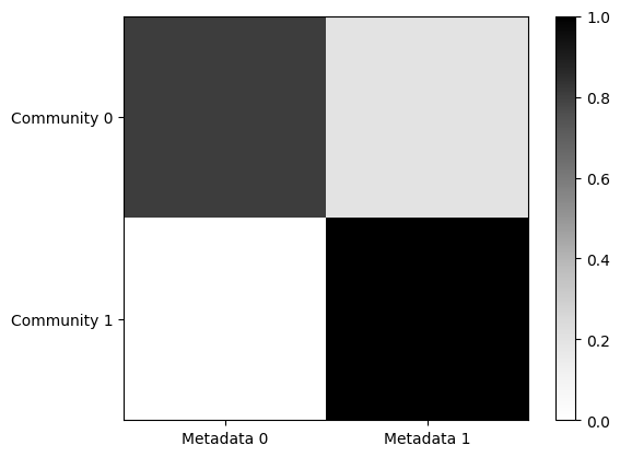
beta is a KxZ dimensional matrix, where Z denotes the total number of different categories
of the node attribute. In this example, the attribute Metadata has 2 categories. Then, every row
k of the beta matrix denotes how much information of the different categories is used to create
the k-th community. Also, this variable is normalized such that every row sums to 1.
plt.imshow(beta, cmap="Greys", interpolation="none", vmin=0, vmax=1)

plt.xticks([0, 1], ["Metadata 0", "Metadata 1"])
plt.yticks([0, 1], ["Community 0", "Community 1"])

plt.colorbar()
plt.show()

Through this plot, we can infer that community 0 is mainly related to nodes with category Metadata 0, while community 1 groups together primarily nodes with the category Metadata 1.
Summary#
This tutorial provides a comprehensive guide on using the probinet package. Specifically, it focuses on the MTCOV algorithm, which is a probabilistic generative model used for network analysis, designed to detect communities within a multilayer network where node attributes are considered.
The tutorial explains the structure of the probinet package, which is organized into several main modules, such as input, models, evaluation, synthetic, model_selection, and utils. It also demonstrates how to configure and run the MTCOV algorithm on the input data imported using the probinet package.
Furthermore, it shows how to analyze the results produced by the model. It explains how to load the inferred parameters from a file, unpack the latent variables, and calculate the out-going hard-memberships. It also shows how to interpret the relationships between communities and attribute categories.
