Decoding Temporal Relationships with DynCRep

Welcome to our tutorial on DynCRep - a cutting-edge tool from the probinet package. Traditional network analysis models often fall short when it comes to capturing the dynamic nature of real-world networks. DynCRep is designed to bridge this gap, providing a robust solution for analyzing and understanding the temporal evolution of complex networks.

The DynCRep (Dynamic Community and Reciprocity) model is a tool that helps us to better understand complex, evolving networks. In real-world scenarios, networks are rarely static. They change and evolve over time, influenced by various factors such as changing relationships, evolving interests, and temporal events. The DynCRep model captures these dynamic interaction patterns by considering the temporal order of connections between pairs of nodes in the network, rather than viewing them independently [SCDB22]. This is a significant departure from standard models, which often assume that the connections between pairs of nodes are independent once we know certain hidden factors. The DynCRep model integrates community structure and reciprocity as key structural information of networks that evolve over time. In this tutorial, we will guide you through the process of applying the DynCRep model to a dynamic network.

NOTE: We suggest the reader to have a basic understanding of the CRep and JointCRep models before diving into this tutorial. If you are not familiar with these methods, we recommend checking out our tutorials CRep algorithm and JointCRep algorithm before proceeding with this one.

Setting the Logger

Let’s first set the logging level to DEBUG so we can see the relevant messages.

# Set logging level to DEBUG
import logging

# Make it be set to DEBUG
logging.getLogger().setLevel(logging.DEBUG)
logging.getLogger("matplotlib").setLevel(logging.WARNING)

Data generation

Before we dive into the tutorial, let’s take a moment to understand the key idea behind the DynCRep model. The DynCRep model considers a temporal network as a sequence of adjacency matrices A where A[t] represents the adjacency matrix of the network at time t. The model takes in the sequence of adjacency matrices A and learns the parameters of the model that best describe the temporal relationships between nodes in the network.

For this tutorial, we will use synthetic data generated using the SyntheticDynCRep class from the probinet synthetic.dynamic module. This is the generative model created using the same modelling assumptions as the DynCRep model. It takes in the parameters:

1. N - The number of nodes in the network.

2. K - The number of communities in the network.

3. T - The number of time steps in the network.

4. avg_degree - The average degree of nodes in the network.

5. structure - The structure of the network.

6. ExpM - The expected number of edges in the network.

7. eta - The reciprocity parameter.

8. corr - The correlation between u and v synthetically generated.

9. over - The fraction of nodes with mixed membership.

10. undirected - Whether the network is undirected.

To gain a deeper understanding of how these parameters influence the model, we can experiment by adjusting some of them and observing the resulting changes. Let’s begin with a straightforward scenario: a network with 50 nodes, divided into 2 communities, observed over a single time step. We’ll set the average degree of the nodes to 5. We’ll then examine the structure of the network when the parameters are set to create an assortative network.

from probinet.synthetic.dynamic import SyntheticDynCRep
import numpy as np

# Set the number of nodes, communities, and time steps
N = 50
K = 2
T = 0  # total number of time steps is T+1
avg_degree = 5

# Structure of the network
structure = "assortative"  # This is the default value

# Fix the rng for reproducibility
rseed = 0
rng = np.random.default_rng(rseed)

# Initialize the synthetic network class
synthetic_dyncrep = SyntheticDynCRep(
    N=N, 
    K=K, 
    T=T, 
    verbose=2, 
    avg_degree=avg_degree, 
    figsize=(3, 3), 
    fontsize=10, 
    rng=rng
)

temporal_network = synthetic_dyncrep.generate_net()

DEBUG:root:------------------------------

DEBUG:root:t=0

DEBUG:root:Number of nodes: 50 
Number of edges: 126

DEBUG:root:Average degree (2E/N): 5.04

DEBUG:root:Reciprocity at t: 0.07936507936507936

DEBUG:root:------------------------------

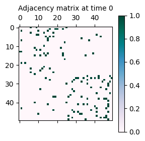
As seen above, the network has been generated with the specified parameters. It consists of 50 nodes clustered into 2 communities. The network is assortative, meaning that nodes are more likely to connect to nodes within the same community. This explains why the adjacency matrix looks like a diagonal-block matrix. Let’s see what happens if the structure is changed to disassortative.

# Structure of the network
structure = "disassortative"

# Fix the rng for reproducibility
rseed = 0
rng = np.random.default_rng(rseed)

# Initialize the synthetic network class
synthetic_dyncrep = SyntheticDynCRep(
    N=N,
    K=K,
    T=T,
    verbose=2,
    avg_degree=avg_degree,
    figsize=(3, 3),
    fontsize=10,
    rng=rng,
    structure=structure,
)

# Generate synthetic dynamic network
temporal_network = synthetic_dyncrep.generate_net()

DEBUG:root:------------------------------

DEBUG:root:t=0

DEBUG:root:Number of nodes: 50 
Number of edges: 126

DEBUG:root:Average degree (2E/N): 5.04

DEBUG:root:Reciprocity at t: 0.12698412698412698

DEBUG:root:------------------------------

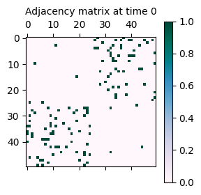
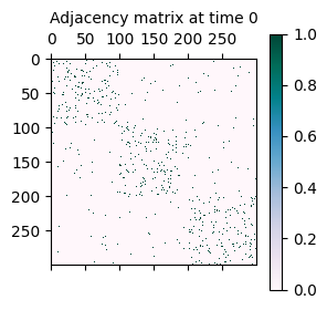
As seen above, the network now has a disassortative structure, meaning that nodes are more likely to connect to nodes in different communities. This is reflected in the adjacency matrix, which has connections off the diagonal.

Notice that the generated network has about 120 edges. If we want to generate a network with a larger number of edges, we can increase the ExpM parameter. Let’s see what happens when we set it to 200.

# Set the expected number of edges
ExpM = 200

# Fix the rng for reproducibility
rseed = 0
rng = np.random.default_rng(rseed)

# Initialize the synthetic network class
synthetic_dyncrep = SyntheticDynCRep(
    N=N,
    K=K,
    T=T,
    verbose=2,
    avg_degree=avg_degree,
    figsize=(3, 3),
    fontsize=10,
    rng=rng,
    structure=structure,
    ExpM=ExpM,
)

# Generate synthetic dynamic network
temporal_network = synthetic_dyncrep.generate_net()

DEBUG:root:------------------------------

DEBUG:root:t=0

DEBUG:root:Number of nodes: 50 
Number of edges: 200

DEBUG:root:Average degree (2E/N): 8.0

DEBUG:root:Reciprocity at t: 0.14

DEBUG:root:------------------------------

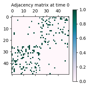
Now the resulting network has about 200 edges, as specified by the ExpM parameter.

Another key element of the DynCRep model is the reciprocity parameter eta. This parameter determines the level of reciprocity in the network, i.e., the likelihood that a connection between two nodes is reciprocated. The difference between this reciprocity parameter and the one introduced in the standard CRep model is that the dependency on the reciprocated tie is on the previous time step, while standard CRep considers only the same time t, being an approach valid for static networks. Let’s see how the network structure changes with different values of eta. By default, the eta parameter is set to 0. Let’s see what happens when we increase to 0.5. Notice that to observe the effect of the reciprocity parameter, we need to generate a network with more than one time step.

# Set the number of time steps
T = 1

# Set the reciprocity parameter
eta = 0.5

# Fix the rng for reproducibility
rseed = 0
rng = np.random.default_rng(rseed)

# Initialize the synthetic network class
synthetic_dyncrep = SyntheticDynCRep(
    N=N,
    K=K,
    T=T,
    verbose=2,
    avg_degree=avg_degree,
    figsize=(3, 3),
    fontsize=10,
    rng=rng,
    eta=eta,
)

# Generate synthetic dynamic network
temporal_network = synthetic_dyncrep.generate_net()

DEBUG:root:------------------------------

DEBUG:root:t=0

DEBUG:root:Number of nodes: 50 
Number of edges: 126

DEBUG:root:Average degree (2E/N): 5.04

DEBUG:root:Reciprocity at t: 0.07936507936507936

DEBUG:root:------------------------------

DEBUG:root:------------------------------

DEBUG:root:t=1

DEBUG:root:Number of nodes: 50 
Number of edges: 131

DEBUG:root:Average degree (2E/N): 5.24

DEBUG:root:Reciprocity at t: 0.22900763358778625

DEBUG:root:------------------------------

DEBUG:root:Compare current and previous reciprocity.

DEBUG:root:Time step: 1

DEBUG:root:Number of non-zero elements in the adjacency matrix at time t: 131.0

DEBUG:root:Fraction of non-zero elements in the transposed adjacency matrix at time t: 0.22900763358778625

DEBUG:root:Fraction of non-zero elements in the transposed adjacency matrix at time t-1: 0.16030534351145037

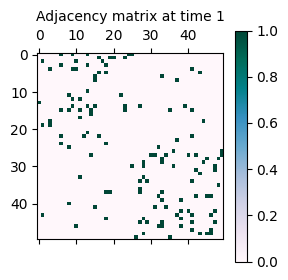
As seen above (more concretely in the graph statistics), the reciprocity in the second time step network is higher than in the first time step network. This is because the eta parameter has been set to 0.5, which increases the likelihood of reciprocated connections in the network. From a graphical perspective, the network structure is more clustered in the second time step, given that the existing connections (i,j) in the first time step are more likely to be reciprocated as (j,i) in the second time step.

Decoding Temporal Relationships with DynCRep

Now that we are more familiar with the generative model, let’s move on to the next step: decoding the temporal relationships in the network using the DynCRep model. For the actual analysis, we will generate a synthetic network with 300 nodes, divided into 3 communities, and observed over 6 time steps. We will set the average degree of the nodes to 10 and the reciprocity parameter to 0.5.

# Set the number of nodes, communities, and time steps
N = 300
K = 3
T = 5
avg_degree = 10
eta = 0.5

# Fix the rng for reproducibility
rseed = 0
rng = np.random.default_rng(rseed)

# Initialize the synthetic network class
synthetic_dyncrep = SyntheticDynCRep(
    N=N,
    K=K,
    T=T,
    verbose=2,
    avg_degree=avg_degree,
    figsize=(3, 3),
    fontsize=10,
    rng=rng,
    eta=eta,
)

# Generate synthetic dynamic network
A = synthetic_dyncrep.generate_net()

DEBUG:root:------------------------------

DEBUG:root:t=0

DEBUG:root:Number of nodes: 300 
Number of edges: 1492

DEBUG:root:Average degree (2E/N): 9.947

DEBUG:root:Reciprocity at t: 0.030831099195710455

DEBUG:root:------------------------------

DEBUG:root:------------------------------

DEBUG:root:t=1

DEBUG:root:Number of nodes: 300 
Number of edges: 1644

DEBUG:root:Average degree (2E/N): 10.96

DEBUG:root:Reciprocity at t: 0.17639902676399027

DEBUG:root:------------------------------

DEBUG:root:------------------------------

DEBUG:root:t=2

DEBUG:root:Number of nodes: 300 
Number of edges: 1760

DEBUG:root:Average degree (2E/N): 11.733

DEBUG:root:Reciprocity at t: 0.2534090909090909

DEBUG:root:------------------------------

DEBUG:root:------------------------------

DEBUG:root:t=3

DEBUG:root:Number of nodes: 300 
Number of edges: 1834

DEBUG:root:Average degree (2E/N): 12.227

DEBUG:root:Reciprocity at t: 0.2791712104689204

DEBUG:root:------------------------------

DEBUG:root:------------------------------

DEBUG:root:t=4

DEBUG:root:Number of nodes: 300 
Number of edges: 1855

DEBUG:root:Average degree (2E/N): 12.367

DEBUG:root:Reciprocity at t: 0.2857142857142857

DEBUG:root:------------------------------

DEBUG:root:------------------------------

DEBUG:root:t=5

DEBUG:root:Number of nodes: 300 
Number of edges: 1912

DEBUG:root:Average degree (2E/N): 12.747

DEBUG:root:Reciprocity at t: 0.3148535564853556

DEBUG:root:------------------------------

DEBUG:root:Compare current and previous reciprocity.

DEBUG:root:Time step: 1

DEBUG:root:Number of non-zero elements in the adjacency matrix at time t: 1644.0

DEBUG:root:Fraction of non-zero elements in the transposed adjacency matrix at time t: 0.17639902676399027

DEBUG:root:Fraction of non-zero elements in the transposed adjacency matrix at time t-1: 0.12347931873479319

DEBUG:root:Time step: 2

DEBUG:root:Number of non-zero elements in the adjacency matrix at time t: 1760.0

DEBUG:root:Fraction of non-zero elements in the transposed adjacency matrix at time t: 0.2534090909090909

DEBUG:root:Fraction of non-zero elements in the transposed adjacency matrix at time t-1: 0.22727272727272727

DEBUG:root:Time step: 3

DEBUG:root:Number of non-zero elements in the adjacency matrix at time t: 1834.0

DEBUG:root:Fraction of non-zero elements in the transposed adjacency matrix at time t: 0.2791712104689204

DEBUG:root:Fraction of non-zero elements in the transposed adjacency matrix at time t-1: 0.26663031624863687

DEBUG:root:Time step: 4

DEBUG:root:Number of non-zero elements in the adjacency matrix at time t: 1855.0

DEBUG:root:Fraction of non-zero elements in the transposed adjacency matrix at time t: 0.2857142857142857

DEBUG:root:Fraction of non-zero elements in the transposed adjacency matrix at time t-1: 0.2857142857142857

DEBUG:root:Time step: 5

DEBUG:root:Number of non-zero elements in the adjacency matrix at time t: 1912.0

DEBUG:root:Fraction of non-zero elements in the transposed adjacency matrix at time t: 0.3148535564853556

DEBUG:root:Fraction of non-zero elements in the transposed adjacency matrix at time t-1: 0.301255230125523

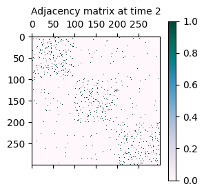
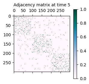
As mentioned initially, the synthetically generated network is a sequence of adjacency matrices A where A[t] represents the adjacency matrix of the network at time t.

A

[<networkx.classes.digraph.DiGraph at 0x7f7ca8a99640>,
 <networkx.classes.digraph.DiGraph at 0x7f7ca8c44140>,
 <networkx.classes.digraph.DiGraph at 0x7f7ca8d86b40>,
 <networkx.classes.digraph.DiGraph at 0x7f7ca8b1f170>,
 <networkx.classes.digraph.DiGraph at 0x7f7ca8b1cc80>,
 <networkx.classes.digraph.DiGraph at 0x7f7ca8b1e2a0>]

To utilize the DynCRep model, we need to transform the sequence of adjacency matrices A into a sequence of adjacency tensors B, where B is a numpy adjacency tensor derived from a NetworkX graph. The build_B_from_A function from the probinet.input.preprocessing module can be used to perform this transformation. The function takes in the sequence of adjacency matrices A and the list of nodes in the network and returns the adjacency tensor B.

from probinet.input.preprocessing import create_adjacency_tensor_from_graph_list

nodes = list(A[0].nodes())
B, _ = create_adjacency_tensor_from_graph_list(A, nodes=nodes)

Done! We now have the adjacency tensor B of dimensions (T+1, N, N) where T is the number of time steps, and N is the number of nodes in the network. The adjacency tensor B is a numpy array that can be used as input to the DynCRep model.

B.shape

(6, 300, 300)

from probinet.models.dyncrep import DynCRep

First, we instantiate the DynCRep model by creating an instance of the class. During this process, we can modify the default attribute values by specifying our desired maximum number of iterations and the number of realizations. The max_iter parameter sets the maximum number of iterations for the optimization algorithm, and the num_realizations parameter defines the number of times the model will run.

dyncrep = DynCRep(max_iter=2000, num_realizations=3)

T = B.shape[0] - 1

The model requires the information to be properly encoded into a GraphData object. We show how to do this below.

from probinet.models.classes import GraphData

# Build the GraphData object to pass to the fit method
gdata = GraphData(
    graph_list=None,
    adjacency_tensor=B,
    transposed_tensor=None,
    nodes=nodes,
    data_values=None,
)

We can now fit the data into the model DynCRep model. We need to set the number of time steps T, the list of nodes in the network, and other parameters too. Given that the data has been generated using K=3, we will change the file to reflect this. The model returns the learned parameters of the model, including the community memberships u, v, the temporal relationships w between the communities, the reciprocity parameter eta, the edge disappearance rate beta and the log-likelihood of the model.

NOTE: The parameters ag and bg are the hyperparameters of the gamma distribution, which is used for regularization. The authors of the main reference assume gamma-distributed priors for the membership vectors. We fix them to 1.1 and 0.5, respectively.

# Fix the rng for reproducibility
rseed = 0
rng = np.random.default_rng(rseed)

u_dyn, v_dyn, w_dyn, eta_dyn, beta_dyn, Loglikelihood_dyn = dyncrep.fit(
    gdata,
    T=T,
    K=K,
    nodes=nodes,
    ag=1.1,
    bg=0.5,
    out_inference=False,
    rng=rng
)

DEBUG:root:Initialization parameter: 0

DEBUG:root:Eta0 parameter: None

INFO:root:### Version: w-DYN ###

DEBUG:root:Number of time steps L: 6

DEBUG:root:T is greater than 0. Proceeding with calculations that require multiple time steps.

DEBUG:root:Random number generator seed: 35399562948360463058890781895381311971

DEBUG:root:eta is initialized randomly.

DEBUG:root:u, v and w are initialized randomly.

DEBUG:root:Updating realization 0 ...

DEBUG:root:num. realization = 0 - iterations = 100 - time = 2.24 seconds

DEBUG:root:num. realization = 0 - iterations = 200 - time = 4.47 seconds

DEBUG:root:num. realization = 0 - iterations = 300 - time = 6.71 seconds

DEBUG:root:num. realization = 0 - iterations = 400 - time = 8.94 seconds

DEBUG:root:num. realization = 0 - iterations = 500 - time = 11.17 seconds

DEBUG:root:num. realization = 0 - iterations = 600 - time = 13.41 seconds

DEBUG:root:num. realization = 0 - iterations = 700 - time = 15.64 seconds

DEBUG:root:num. realizations = 0 - Log-likelihood = -23086.767217859804 - iterations = 721 - time = 16.12 seconds - convergence = True

DEBUG:root:Random number generator seed: 203178491105477591223103010971659415971

DEBUG:root:eta is initialized randomly.

DEBUG:root:u, v and w are initialized randomly.

DEBUG:root:Updating realization 1 ...

DEBUG:root:num. realization = 1 - iterations = 100 - time = 2.24 seconds

DEBUG:root:num. realization = 1 - iterations = 200 - time = 4.49 seconds

DEBUG:root:num. realization = 1 - iterations = 300 - time = 6.74 seconds

DEBUG:root:num. realization = 1 - iterations = 400 - time = 8.98 seconds

DEBUG:root:num. realization = 1 - iterations = 500 - time = 11.23 seconds

DEBUG:root:num. realization = 1 - iterations = 600 - time = 13.48 seconds

DEBUG:root:num. realization = 1 - iterations = 700 - time = 15.73 seconds

DEBUG:root:num. realization = 1 - iterations = 800 - time = 17.98 seconds

DEBUG:root:num. realization = 1 - iterations = 900 - time = 20.24 seconds

DEBUG:root:num. realizations = 1 - Log-likelihood = -23538.732583283192 - iterations = 981 - time = 22.09 seconds - convergence = True

DEBUG:root:Random number generator seed: 118970195796093957196501181087388680547

DEBUG:root:eta is initialized randomly.

DEBUG:root:u, v and w are initialized randomly.

DEBUG:root:Updating realization 2 ...

DEBUG:root:num. realization = 2 - iterations = 100 - time = 2.24 seconds

DEBUG:root:num. realization = 2 - iterations = 200 - time = 4.49 seconds

DEBUG:root:num. realization = 2 - iterations = 300 - time = 6.72 seconds

DEBUG:root:num. realization = 2 - iterations = 400 - time = 8.96 seconds

DEBUG:root:num. realization = 2 - iterations = 500 - time = 11.18 seconds

DEBUG:root:num. realization = 2 - iterations = 600 - time = 13.41 seconds

DEBUG:root:num. realizations = 2 - Log-likelihood = -23134.291440811314 - iterations = 621 - time = 13.88 seconds - convergence = True

DEBUG:root:Best realization = 0 - maxL = -23086.767217859804 - best iterations = 721

INFO:root:Algorithm successfully converged after 721 iterations with a maximum log-likelihood of -23086.7672.

DEBUG:root:Parameters won't be saved! If you want to save them, set out_inference=True.

The DynCRep model has been effectively applied to the adjacency tensor B, with the fitting process carried out over three realizations, all of which achieved successful convergence. As detailed in the referenced paper and other tutorials, the vectors u and v represent the out-going and in-coming community memberships of the network’s nodes, respectively, and remain constant over time. Conversely, the affinity matrix, which delineates the edge density within and between communities, is a time-dependent function. By utilizing the plot_matrices function outlined below, we can observe the evolution of these relationships over time.

NOTE: You might be curious as to why the parameters u and v remain constant over time. As outlined in the primary reference, it’s not necessary to estimate these parameters at every time step. The model is designed to estimate them just once. This represents a first approach, where the affinity matrix is treated as a time-dependent variable, while the community membership vectors, u and v, are kept static over time. It’s worth noting that an alternative interpretation could involve fixing w and allowing u and v to change over time. As explained by the authors, the model can be easily adapted to accommodate this alternative scenario.

w_dyn.shape

(6, 3, 3)

# Set the colormap for the plots
cmap = "PuBuGn"
import matplotlib.pyplot as plt
from matplotlib.colors import Normalize


def plot_matrices(w, cmap="PuBuGn"):
    """
    Plot a temporal array in a row of subplots with a single shared colorbar.

    Parameters
    ----------
    w : np.ndarray
        Temporal array to plot.
    cmap : str, optional
        Colormap to use for the plots. Default is 'PuBuGn'.
    """
    # Get the number of time steps
    T = w.shape[0]

    # Normalize the data for consistent color mapping
    norm = Normalize(vmin=np.min(w), vmax=np.max(w))

    # Create a new figure with specified size
    fig, axes = plt.subplots(1, T, figsize=(3 * T, 3), constrained_layout=True)

    # Loop over each time step
    for t in range(T):
        # Add a subplot for the current time step
        if T == 1:
            ax = axes
        else:
            ax = axes[t]

        # Display the matrix as an image
        cax = ax.imshow(
            w[t], cmap=cmap, norm=norm, interpolation="nearest", extent=[0, 3, 0, 3]
        )

        # Add a title to the subplot
        ax.set_title("Time step: " + str(t), fontsize=18)

        # Set ticks to be at 0.5, 1.5, 2.5 but show as 0, 1, 2
        ax.set_xticks([0.5, 1.5, 2.5])
        ax.set_yticks([0.5, 1.5, 2.5])

        # Set tick labels to 0, 1, 2
        ax.set_xticklabels([0, 1, 2])
        ax.set_yticklabels([2, 1, 0])

    # Add a single colorbar to the figure
    fig.colorbar(cax, ax=axes, orientation="vertical", fraction=0.046, pad=0.04)

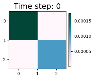
plot_matrices(w_dyn)

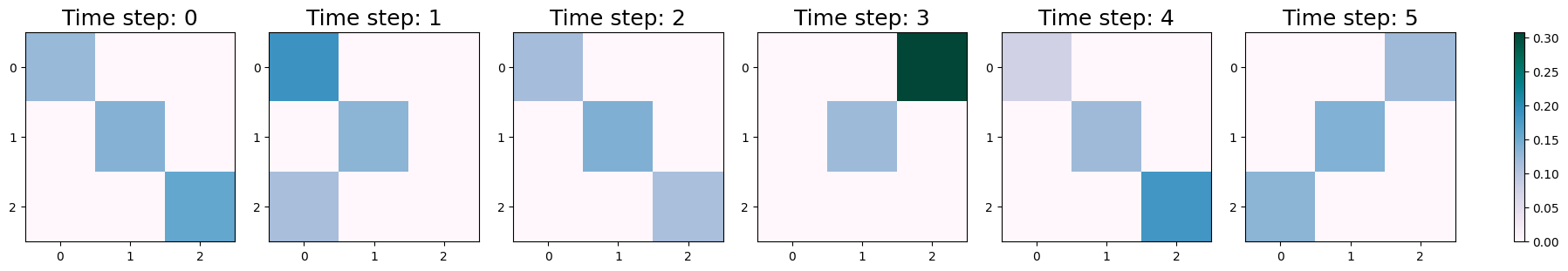
The interactions between communities vary across different timesteps, as depicted in the visualizations. These interactions, in conjunction with the vectors u and v, provide insights into the temporal evolution of community memberships.

To further our understanding, we can compare the inferred expected adjacency tensor with the input data used to train the model.

from probinet.evaluation.expectation_computation import (
    compute_expected_adjacency_tensor_multilayer,
)
from probinet.utils.matrix_operations import transpose_tensor

# Define the number of time steps
T = B.shape[0] - 1

# Compute the expected adjacency tensor
lambda_inf_dyn = compute_expected_adjacency_tensor_multilayer(u_dyn, v_dyn, w_dyn)
M_inf_dyn = lambda_inf_dyn + eta_dyn * transpose_tensor(B)

The comparison between the two temporal arrays can be done using the calculate_AUC function from the probinet.evaluation module. This function calculates the Area Under the Curve (AUC) for the given temporal arrays. We can use this function to compute the AUC for each time step, i.e., the probability that a randomly selected edge has higher expected value than a randomly selected non-existing edge. A value of 1 means perfect reconstruction, while 0.5 is pure random chance.

from probinet.evaluation.link_prediction import compute_link_prediction_AUC
from probinet.utils.tools import flt

# Compute the AUC for each time step
for t in range(T + 1):
    print(
        f"Time step {t}: AUC = {flt(compute_link_prediction_AUC(B[t].astype('int'), M_inf_dyn[t]))}"
    )

Time step 0: AUC = 0.783
Time step 1: AUC = 0.747
Time step 2: AUC = 0.82
Time step 3: AUC = 0.771
Time step 4: AUC = 0.813
Time step 5: AUC = 0.796

As we can see, the results obtained from the DynCRep model show a high AUC value for each time. We can also get a graphical feeling about how the inferred temporal relationships compare to the input data by using the plot_temporal_arrays function defined below.

def plot_temporal_arrays(arrays, titles=None, cmap="PuBuGn"):
    """
    Plot a list of temporal arrays in separate columns.

    Parameters
    ----------
    arrays : list of np.ndarray
        List of temporal arrays to plot.
    cmap : str, optional
        Colormap to use for the plots. Default is 'PuBuGn'.
    """
    # Get the number of time steps from the first array in the list
    T = arrays[0].shape[0] - 1

    # Create a new figure with specified size
    plt.figure(figsize=(3 * len(arrays), 10))

    # Loop over each time step
    for t in range(T + 1):
        # Loop over each array
        for i, array in enumerate(arrays):
            # Add a subplot for the current array at the current time step
            plt.subplot(T + 1, len(arrays), i + len(arrays) * t + 1)

            # Display the array as an image
            plt.imshow(array[t], cmap=cmap, interpolation="nearest")

            # Add a colorbar to the plot
            plt.colorbar(fraction=0.046)

            # Add a title to the first subplot of each column
            if t == 0:
                if titles is not None:
                    plt.title(titles[i])
                else:
                    plt.title(f"Array {i + 1}")

plot_temporal_arrays([B, M_inf_dyn], titles=["Input Data", "DynCRep-Dynamic \nExpectation"])

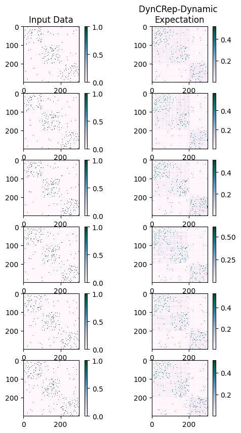
As detailed in the main reference [SCDB22], the DynCRep algorithm operates in two distinct modes: Dynamic and Static. The Dynamic mode (also known as w-DYN), which is the default setting, captures and stores temporal relationships in a time-dependent affinity matrix, allowing for a nuanced understanding of evolving community structures. On the other hand, the Static mode (also known as w-STATIC), despite u, v and w being fixed in time, still allows for network evolution. This is facilitated by the appearance and disappearance of edges, governed by the parameters beta and eta. These two modes enhance the flexibility of the model, enabling it to effectively handle a variety of community structures.

Let’s see now how to use the Static mode of the DynCRep model to decode the temporal relationships in the network. We will use the same synthetic network generated earlier, but this time we will fit the DynCRep model in Static mode by setting the temporal parameter to False.

# Fix the rng for reproducibility
rseed = 0
rng = np.random.default_rng(rseed)

u_stat, v_stat, w_stat, eta_stat, beta_stat, Loglikelihood = dyncrep.fit(
    gdata,
    T=T,
    flag_data_T=0,
    ag=1.1,
    bg=0.5,
    temporal=False,  # <- Static mode
    out_inference=False,
    rng=rng
)

DEBUG:root:Initialization parameter: 0

DEBUG:root:Eta0 parameter: None

INFO:root:### Version: w-STATIC ###

DEBUG:root:Number of time steps L: 1

DEBUG:root:T is greater than 0. Proceeding with calculations that require multiple time steps.

DEBUG:root:Random number generator seed: 35399562948360463058890781895381311971

DEBUG:root:eta is initialized randomly.

DEBUG:root:u, v and w are initialized randomly.

DEBUG:root:Updating realization 0 ...

DEBUG:root:num. realization = 0 - iterations = 100 - time = 0.30 seconds

DEBUG:root:num. realization = 0 - iterations = 200 - time = 0.59 seconds

DEBUG:root:num. realizations = 0 - Log-likelihood = -26646.376511830265 - iterations = 231 - time = 0.69 seconds - convergence = True

DEBUG:root:Random number generator seed: 146102082068021069584449920474084771037

DEBUG:root:eta is initialized randomly.

DEBUG:root:u, v and w are initialized randomly.

DEBUG:root:Updating realization 1 ...

DEBUG:root:num. realization = 1 - iterations = 100 - time = 0.29 seconds

DEBUG:root:num. realization = 1 - iterations = 200 - time = 0.59 seconds

DEBUG:root:num. realization = 1 - iterations = 300 - time = 0.88 seconds

DEBUG:root:num. realizations = 1 - Log-likelihood = -26646.376511293165 - iterations = 301 - time = 0.89 seconds - convergence = True

DEBUG:root:Random number generator seed: 268373513923159823696334402928712542503

DEBUG:root:eta is initialized randomly.

DEBUG:root:u, v and w are initialized randomly.

DEBUG:root:Updating realization 2 ...

DEBUG:root:num. realization = 2 - iterations = 100 - time = 0.29 seconds

DEBUG:root:num. realization = 2 - iterations = 200 - time = 0.59 seconds

DEBUG:root:num. realization = 2 - iterations = 300 - time = 0.89 seconds

DEBUG:root:num. realizations = 2 - Log-likelihood = -26690.222819729777 - iterations = 311 - time = 0.92 seconds - convergence = True

DEBUG:root:Best realization = 1 - maxL = -26646.376511293165 - best iterations = 301

INFO:root:Algorithm successfully converged after 301 iterations with a maximum log-likelihood of -26646.3765.

DEBUG:root:Parameters won't be saved! If you want to save them, set out_inference=True.

As shown before, the affinity matrix w is now a constant matrix.

plot_matrices(w_stat)

Summary

We have shown this way how to use the DynCRep model to decode the temporal relationships in a network. The model provides a powerful framework for understanding the dynamic nature of complex networks, capturing the temporal evolution of community structures and reciprocity. We hope this tutorial has provided you with a solid foundation for working with the DynCRep model and decoding temporal relationships in dynamic networks.