Cross-Validation And Anomaly Detection With The ACD Algorithm#
Welcome to our tutorial on the Anomaly and Community Detection (ACD) method. This is a
probabilistic
generative model and efficient algorithm to model anomalous edges in networks. It assigns latent
variables as community memberships to nodes and anomaly to the edges [SDB22].
In this tutorial, we will demonstrate how to use the ACD method. We will start by loading the data, performing cross-validation using the model_selection submodule, and then analyzing the results to determine the best number of communities K.
Setting the Logger#
Let’s first set the logging level to DEBUG so we can see the relevant messages.
# Set logging level to DEBUG
import logging

# Make it be set to DEBUG
logging.basicConfig(level=logging.DEBUG)
logging.getLogger("matplotlib").setLevel(logging.WARNING)
Loading and Visualizing the Data#
In this section, we will load the synthetic data required for our analyses. We will start by
importing the necessary libraries and defining the file path for the adjacency matrix, and then,
we will use the build_adjacency_from_file method to read it.
# Step 1: Load the Data
from probinet.input.loader import build_adjacency_from_file

from importlib.resources import files

# Import necessary libraries
import pandas as pd

# Define the adjacency file
adj_file = "synthetic_network_with_anomalies.dat"

# Load the network data
with files("probinet.data.input").joinpath(adj_file).open("rb") as network:
    graph_data = build_adjacency_from_file(network.name, header=0)
DEBUG:root:Read adjacency file from /home/runner/.local/lib/python3.12/site-packages/probinet/data/input/synthetic_network_with_anomalies.dat. The shape of the data is (5459, 3).
DEBUG:root:Creating the networks ...
DEBUG:root:Removing self loops
Number of nodes = 500
Number of layers = 1
Number of edges and average degree in each layer:
E[0] = 5459 / <k> = 21.84
Sparsity [0] = 0.022
Reciprocity (networkX) = 0.077
Reciprocity (considering the weights of the edges) = 0.077
As we have seen in previous tutorials, the build_adjacency_from_file outputs a list of MultiDiGraph NetworkX
objects, a graph adjacency tensor B, a transposed graph adjacency tensor B_T, and
an array with values of entries A[j, i] given non-zero entry (i, j). These outputs are
essential for analyzing the network structure and performing further computations.
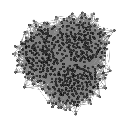
Now that we have loaded the data, we can proceed to visualize the network structure.
import matplotlib.pyplot as plt
import networkx as nx

# Extract the graph list
A = graph_data.graph_list

# Set the seed for the layout
pos = nx.spring_layout(A[0], seed=42)

# Draw the graph using the spring layout
plt.figure(figsize=(5, 5))
nx.draw(
    A[0],
    pos=pos,
    node_size=50,
    node_color="black",
    alpha=0.6,
    edge_color="gray",
    with_labels=False,
)
plt.show()
Performing the Cross-Validation#
As we can see from the plot, there’s no clear clustering. However, we can use the
ACD algorithm to infer the communities, and also to get some
information about the anomalies. To do this, we need to specify a set of parameters related to the number of communities, their interrelations, and other structural aspects. Selecting the appropriate hyperparameters can be challenging, so we will utilize the model_selection module, which is designed for model selection and cross-validation to optimize the algorithm’s performance.
The model_selection module not only provides a comprehensive set of tools for model selection and cross-validation but also enables us to build specific modules for each model that carry out the cross-validation process. This module includes several submodules, each tailored for specific tasks:
parameter_search: Functions for searching optimal model parameters.cross_validation: Functions for general cross-validation.masking: Functions for masking data during cross-validation.main: Entry point for the cross-validation process. Although each algorithm has its own cross-validation submodule, themainsubmodule provides a unified interface for running cross-validation for all algorithms.
Additionally, the module provides specialized cross-validation submodules for different algorithms:
mtcov_cross_validation: Cross-validation specific to theMTCOValgorithm.dyncrep_cross_validation: Cross-validation specific to theDynCRepalgorithm.acd_cross_validation: Cross-validation specific to theACDalgorithm.crep_cross_validation: Cross-validation specific to theCRepalgorithm.jointcrep_cross_validation: Cross-validation specific to theJointCRepalgorithm.
By leveraging these tools, we can systematically assess and fine-tune our model to achieve the best possible results.
Let’s look now at how to use it. As mentioned, we will use the main submodule to perform
cross-validation for the ACD method. To do that, we need to define the model parameters
(model_parameters) and cross-validation parameters (cv_params). The model_parameters
include the lists of hyperparameters of the ACD method we would like to test. The cv_params
include the parameters for the cross-validation process, such as the number of folds, the input
folder, and the output results. Optionally, we can also specify another dictionary
(numerical_parameters) with the
numerical parameters to run the inference algorithm, like the number of iterations or the
convergence threshold. We will set the number of iterations to 1000 using this input dictionary.
# Step 2: Perform Cross-Validation
fold_number = 3
# Define the cross-validation parameters
model_parameters = {
    "K": [2, 3],
    "flag_anomaly": True,
    "rseed": 10,
    "initialization": 0,
    "out_inference": False,
    "out_folder": "tutorial_outputs/ACD/" + str(fold_number) + "-fold_cv/",
    "end_file": "_ACD",
    "assortative": True,
    "undirected": False,
    "files": "",
}
cv_params = {
    "in_folder": "../../../probinet/data/input/",
    "adj": adj_file,
    "ego": "source",
    "alter": "target",
    "NFold": fold_number,
    "out_results": True,
    "out_mask": False,
    "sep": " ",
}
numerical_parameters = {
    "max_iter": 1000,
    "num_realizations": 1,
}
As we can see, the model_parameters dictionary contains the hyperparameters we want to test. In
this case, we will only focus on the number of communities K. To avoid making the tutorial too long, we will only test two values for K, but in practice, we should test a broader range of values.
We are now ready to run the cross-validation process. We will use the cross_validation function from the main submodule, passing the method name (ACD), the model parameters, and the cross-validation parameters as arguments. The function will then perform the cross-validation and store the results in a CSV file.
from pathlib import Path

# Define the output file name
adj_file_stem = Path(adj_file).stem
cv_results_file = Path(f"outputs/{fold_number}-fold_cv/{adj_file_stem}_cv.csv")

# Delete the file if it already exists
if cv_results_file.exists():
    cv_results_file.unlink()

# Run the cross-validation
from probinet.model_selection.main import cross_validation

results = cross_validation("ACD", model_parameters, cv_params, numerical_parameters)
INFO:root:Starting cross-validation for algorithm: ACD
DEBUG:root:Converting parameter flag_anomaly to list. The value used is True
DEBUG:root:Converting parameter rseed to list. The value used is 10
DEBUG:root:Converting parameter initialization to list. The value used is 0
DEBUG:root:Converting parameter out_inference to list. The value used is False
DEBUG:root:Converting parameter out_folder to list. The value used is tutorial_outputs/ACD/3-fold_cv/
DEBUG:root:Converting parameter end_file to list. The value used is _ACD
DEBUG:root:Converting parameter assortative to list. The value used is True
DEBUG:root:Converting parameter undirected to list. The value used is False
DEBUG:root:Converting parameter files to list. The value used is
INFO:root:Parameter grid created with 2 combinations
INFO:root:Running cross-validation for parameters: {'K': 2, 'flag_anomaly': True, 'rseed': 10, 'initialization': 0, 'out_inference': False, 'out_folder': 'tutorial_outputs/ACD/3-fold_cv/', 'end_file': '_ACD', 'assortative': True, 'undirected': False, 'files': ''}
INFO:root:Results will be saved in: tutorial_outputs/ACD/3-fold_cv/synthetic_network_with_anomalies_cv.csv
DEBUG:root:Read adjacency file from ../../../probinet/data/input/synthetic_network_with_anomalies.dat. The shape of the data is (5459, 3).
DEBUG:root:Creating the networks ...
DEBUG:root:Removing self loops
INFO:root:Starting the cross-validation procedure.
INFO:root:
FOLD 0
DEBUG:root:Initialization parameter: 0
DEBUG:root:Eta0 parameter: None
DEBUG:root:Preprocessing the data for fitting the models.
DEBUG:root:Data looks like: [[[0. 0. 0. ... 0. 0. 0.]
  [0. 0. 0. ... 0. 0. 0.]
  [0. 0. 0. ... 1. 0. 0.]
  ...
  [0. 1. 0. ... 0. 0. 0.]
  [0. 0. 0. ... 0. 0. 0.]
  [0. 0. 0. ... 0. 0. 0.]]]
DEBUG:root:Random number generator state: 32318217809460493494586234015929749787
DEBUG:root:u, v and w are initialized randomly.
DEBUG:root:Updating realization 0 ...
Number of nodes = 500
Number of layers = 1
Number of edges and average degree in each layer:
E[0] = 5459 / <k> = 21.84
Sparsity [0] = 0.022
Reciprocity (networkX) = 0.077
Reciprocity (considering the weights of the edges) = 0.077
DEBUG:root:num. realization = 0 - iterations = 100 - time = 4.42 seconds
DEBUG:root:num. realization = 0 - iterations = 200 - time = 8.80 seconds
DEBUG:root:num. realization = 0 - iterations = 300 - time = 13.17 seconds
DEBUG:root:num. realization = 0 - iterations = 400 - time = 17.54 seconds
DEBUG:root:num. realization = 0 - iterations = 500 - time = 21.91 seconds
DEBUG:root:num. realization = 0 - iterations = 600 - time = 26.30 seconds
DEBUG:root:num. realization = 0 - iterations = 700 - time = 30.68 seconds
DEBUG:root:num. realization = 0 - iterations = 800 - time = 35.08 seconds
DEBUG:root:num. realization = 0 - iterations = 900 - time = 39.50 seconds
DEBUG:root:num. realization = 0 - iterations = 1000 - time = 43.92 seconds
DEBUG:root:num. realizations = 0 - ELBO = -23424.339552468733 - ELBOmax = -23424.339552468733 - iterations = 1000 - time = 43.92 seconds - convergence = False
DEBUG:root:Best realization = 0 - maxL = -23424.339552468733 - best iterations = 1000
INFO:root:Algorithm did not converge.
WARNING:root:Solution failed to converge in 1000 EM steps!
WARNING:root:Parameters won't be saved for this realization! If you have provided a number of realizations equal to one, please increase it.
INFO:root:Time elapsed: 44.04 seconds.
INFO:root:
Time elapsed: 44.04 seconds.
INFO:root:
FOLD 1
DEBUG:root:Initialization parameter: 0
DEBUG:root:Eta0 parameter: None
DEBUG:root:Preprocessing the data for fitting the models.
DEBUG:root:Data looks like: [[[0. 0. 0. ... 0. 0. 0.]
  [0. 0. 0. ... 0. 0. 0.]
  [0. 0. 0. ... 0. 0. 0.]
  ...
  [0. 1. 1. ... 0. 0. 0.]
  [0. 0. 0. ... 0. 0. 0.]
  [0. 0. 0. ... 0. 0. 0.]]]
DEBUG:root:Random number generator state: 32318217809460493494586234015929749787
DEBUG:root:u, v and w are initialized randomly.
DEBUG:root:Updating realization 0 ...
DEBUG:root:num. realization = 0 - iterations = 100 - time = 4.43 seconds
DEBUG:root:num. realization = 0 - iterations = 200 - time = 8.84 seconds
DEBUG:root:num. realization = 0 - iterations = 300 - time = 13.27 seconds
DEBUG:root:num. realization = 0 - iterations = 400 - time = 17.71 seconds
DEBUG:root:num. realization = 0 - iterations = 500 - time = 22.11 seconds
DEBUG:root:num. realization = 0 - iterations = 600 - time = 26.52 seconds
DEBUG:root:num. realization = 0 - iterations = 700 - time = 30.91 seconds
DEBUG:root:num. realization = 0 - iterations = 800 - time = 35.32 seconds
DEBUG:root:num. realization = 0 - iterations = 900 - time = 39.74 seconds
DEBUG:root:num. realization = 0 - iterations = 1000 - time = 44.14 seconds
DEBUG:root:num. realizations = 0 - ELBO = -22548.27344323408 - ELBOmax = -22548.27344323408 - iterations = 1000 - time = 44.14 seconds - convergence = False
DEBUG:root:Best realization = 0 - maxL = -22548.27344323408 - best iterations = 1000
INFO:root:Algorithm did not converge.
WARNING:root:Solution failed to converge in 1000 EM steps!
WARNING:root:Parameters won't be saved for this realization! If you have provided a number of realizations equal to one, please increase it.
INFO:root:Time elapsed: 44.24 seconds.
INFO:root:
Time elapsed: 88.29 seconds.
INFO:root:
FOLD 2
DEBUG:root:Initialization parameter: 0
DEBUG:root:Eta0 parameter: None
DEBUG:root:Preprocessing the data for fitting the models.
DEBUG:root:Data looks like: [[[0. 0. 0. ... 0. 0. 0.]
  [0. 0. 0. ... 0. 0. 0.]
  [0. 0. 0. ... 1. 0. 0.]
  ...
  [0. 0. 1. ... 0. 0. 0.]
  [0. 0. 0. ... 0. 0. 0.]
  [0. 0. 0. ... 0. 0. 0.]]]
DEBUG:root:Random number generator state: 32318217809460493494586234015929749787
DEBUG:root:u, v and w are initialized randomly.
DEBUG:root:Updating realization 0 ...
DEBUG:root:num. realization = 0 - iterations = 100 - time = 4.40 seconds
DEBUG:root:num. realization = 0 - iterations = 200 - time = 8.81 seconds
DEBUG:root:num. realization = 0 - iterations = 300 - time = 13.20 seconds
DEBUG:root:num. realization = 0 - iterations = 400 - time = 17.60 seconds
DEBUG:root:num. realization = 0 - iterations = 500 - time = 21.99 seconds
DEBUG:root:num. realization = 0 - iterations = 600 - time = 26.40 seconds
DEBUG:root:num. realization = 0 - iterations = 700 - time = 30.82 seconds
DEBUG:root:num. realization = 0 - iterations = 800 - time = 35.21 seconds
DEBUG:root:num. realization = 0 - iterations = 900 - time = 39.62 seconds
DEBUG:root:num. realization = 0 - iterations = 1000 - time = 44.06 seconds
DEBUG:root:num. realizations = 0 - ELBO = -23364.426988026218 - ELBOmax = -23364.426988026218 - iterations = 1000 - time = 44.06 seconds - convergence = False
DEBUG:root:Best realization = 0 - maxL = -23364.426988026218 - best iterations = 1000
INFO:root:Algorithm did not converge.
WARNING:root:Solution failed to converge in 1000 EM steps!
WARNING:root:Parameters won't be saved for this realization! If you have provided a number of realizations equal to one, please increase it.
INFO:root:Time elapsed: 44.17 seconds.
INFO:root:
Time elapsed: 132.46 seconds.
INFO:root:Completed cross-validation for parameters: {'K': 2, 'flag_anomaly': True, 'rseed': 10, 'initialization': 0, 'out_inference': False, 'out_folder': 'tutorial_outputs/ACD/3-fold_cv/', 'end_file': '_ACD_2K2', 'assortative': True, 'undirected': False, 'files': '', 'rng': Generator(PCG64) at 0x7F0206321540}
INFO:root:Running cross-validation for parameters: {'K': 3, 'flag_anomaly': True, 'rseed': 10, 'initialization': 0, 'out_inference': False, 'out_folder': 'tutorial_outputs/ACD/3-fold_cv/', 'end_file': '_ACD', 'assortative': True, 'undirected': False, 'files': ''}
INFO:root:Results will be saved in: tutorial_outputs/ACD/3-fold_cv/synthetic_network_with_anomalies_cv.csv
DEBUG:root:Read adjacency file from ../../../probinet/data/input/synthetic_network_with_anomalies.dat. The shape of the data is (5459, 3).
DEBUG:root:Creating the networks ...
DEBUG:root:Removing self loops
INFO:root:Starting the cross-validation procedure.
INFO:root:
FOLD 0
DEBUG:root:Initialization parameter: 0
DEBUG:root:Eta0 parameter: None
DEBUG:root:Preprocessing the data for fitting the models.
DEBUG:root:Data looks like: [[[0. 0. 0. ... 0. 0. 0.]
  [0. 0. 0. ... 0. 0. 0.]
  [0. 0. 0. ... 1. 0. 0.]
  ...
  [0. 1. 0. ... 0. 0. 0.]
  [0. 0. 0. ... 0. 0. 0.]
  [0. 0. 0. ... 0. 0. 0.]]]
DEBUG:root:Random number generator state: 32318217809460493494586234015929749787
DEBUG:root:u, v and w are initialized randomly.
DEBUG:root:Updating realization 0 ...
Number of nodes = 500
Number of layers = 1
Number of edges and average degree in each layer:
E[0] = 5459 / <k> = 21.84
Sparsity [0] = 0.022
Reciprocity (networkX) = 0.077
Reciprocity (considering the weights of the edges) = 0.077
DEBUG:root:num. realization = 0 - iterations = 100 - time = 4.60 seconds
DEBUG:root:num. realization = 0 - iterations = 200 - time = 9.19 seconds
DEBUG:root:num. realization = 0 - iterations = 300 - time = 13.76 seconds
DEBUG:root:num. realization = 0 - iterations = 400 - time = 18.49 seconds
DEBUG:root:num. realization = 0 - iterations = 500 - time = 23.17 seconds
DEBUG:root:num. realization = 0 - iterations = 600 - time = 27.78 seconds
DEBUG:root:num. realization = 0 - iterations = 700 - time = 32.37 seconds
DEBUG:root:num. realization = 0 - iterations = 800 - time = 36.96 seconds
DEBUG:root:num. realization = 0 - iterations = 900 - time = 41.55 seconds
DEBUG:root:num. realization = 0 - iterations = 1000 - time = 46.10 seconds
DEBUG:root:num. realizations = 0 - ELBO = -24429.988487268485 - ELBOmax = -24429.988487268485 - iterations = 1000 - time = 46.1 seconds - convergence = False
DEBUG:root:Best realization = 0 - maxL = -24429.988487268485 - best iterations = 1000
INFO:root:Algorithm did not converge.
WARNING:root:Solution failed to converge in 1000 EM steps!
WARNING:root:Parameters won't be saved for this realization! If you have provided a number of realizations equal to one, please increase it.
INFO:root:Time elapsed: 46.21 seconds.
INFO:root:
Time elapsed: 46.22 seconds.
INFO:root:
FOLD 1
DEBUG:root:Initialization parameter: 0
DEBUG:root:Eta0 parameter: None
DEBUG:root:Preprocessing the data for fitting the models.
DEBUG:root:Data looks like: [[[0. 0. 0. ... 0. 0. 0.]
  [0. 0. 0. ... 0. 0. 0.]
  [0. 0. 0. ... 0. 0. 0.]
  ...
  [0. 1. 1. ... 0. 0. 0.]
  [0. 0. 0. ... 0. 0. 0.]
  [0. 0. 0. ... 0. 0. 0.]]]
DEBUG:root:Random number generator state: 32318217809460493494586234015929749787
DEBUG:root:u, v and w are initialized randomly.
DEBUG:root:Updating realization 0 ...
DEBUG:root:num. realization = 0 - iterations = 100 - time = 4.60 seconds
DEBUG:root:num. realization = 0 - iterations = 200 - time = 9.21 seconds
DEBUG:root:num. realization = 0 - iterations = 300 - time = 13.81 seconds
DEBUG:root:num. realization = 0 - iterations = 400 - time = 18.41 seconds
DEBUG:root:num. realization = 0 - iterations = 500 - time = 22.99 seconds
DEBUG:root:num. realization = 0 - iterations = 600 - time = 27.58 seconds
DEBUG:root:num. realization = 0 - iterations = 700 - time = 32.18 seconds
DEBUG:root:num. realization = 0 - iterations = 800 - time = 36.80 seconds
DEBUG:root:num. realization = 0 - iterations = 900 - time = 41.45 seconds
DEBUG:root:num. realization = 0 - iterations = 1000 - time = 46.12 seconds
DEBUG:root:num. realizations = 0 - ELBO = -24077.26218072588 - ELBOmax = -24077.26218072588 - iterations = 1000 - time = 46.12 seconds - convergence = False
DEBUG:root:Best realization = 0 - maxL = -24077.26218072588 - best iterations = 1000
INFO:root:Algorithm did not converge.
WARNING:root:Solution failed to converge in 1000 EM steps!
WARNING:root:Parameters won't be saved for this realization! If you have provided a number of realizations equal to one, please increase it.
INFO:root:Time elapsed: 46.22 seconds.
INFO:root:
Time elapsed: 92.44 seconds.
INFO:root:
FOLD 2
DEBUG:root:Initialization parameter: 0
DEBUG:root:Eta0 parameter: None
DEBUG:root:Preprocessing the data for fitting the models.
DEBUG:root:Data looks like: [[[0. 0. 0. ... 0. 0. 0.]
  [0. 0. 0. ... 0. 0. 0.]
  [0. 0. 0. ... 1. 0. 0.]
  ...
  [0. 0. 1. ... 0. 0. 0.]
  [0. 0. 0. ... 0. 0. 0.]
  [0. 0. 0. ... 0. 0. 0.]]]
DEBUG:root:Random number generator state: 32318217809460493494586234015929749787
DEBUG:root:u, v and w are initialized randomly.
DEBUG:root:Updating realization 0 ...
DEBUG:root:num. realization = 0 - iterations = 100 - time = 4.65 seconds
DEBUG:root:num. realization = 0 - iterations = 200 - time = 9.31 seconds
DEBUG:root:num. realization = 0 - iterations = 300 - time = 13.93 seconds
DEBUG:root:num. realization = 0 - iterations = 400 - time = 18.54 seconds
DEBUG:root:num. realization = 0 - iterations = 500 - time = 23.13 seconds
DEBUG:root:num. realization = 0 - iterations = 600 - time = 27.73 seconds
DEBUG:root:num. realization = 0 - iterations = 700 - time = 32.37 seconds
DEBUG:root:num. realization = 0 - iterations = 800 - time = 36.99 seconds
DEBUG:root:num. realization = 0 - iterations = 900 - time = 41.61 seconds
DEBUG:root:num. realization = 0 - iterations = 1000 - time = 46.20 seconds
DEBUG:root:num. realizations = 0 - ELBO = -24422.63280529732 - ELBOmax = -24422.63280529732 - iterations = 1000 - time = 46.2 seconds - convergence = False
DEBUG:root:Best realization = 0 - maxL = -24422.63280529732 - best iterations = 1000
INFO:root:Algorithm did not converge.
WARNING:root:Solution failed to converge in 1000 EM steps!
WARNING:root:Parameters won't be saved for this realization! If you have provided a number of realizations equal to one, please increase it.
INFO:root:Time elapsed: 46.31 seconds.
INFO:root:
Time elapsed: 138.75 seconds.
INFO:root:Completed cross-validation for parameters: {'K': 3, 'flag_anomaly': True, 'rseed': 10, 'initialization': 0, 'out_inference': False, 'out_folder': 'tutorial_outputs/ACD/3-fold_cv/', 'end_file': '_ACD_2K3', 'assortative': True, 'undirected': False, 'files': '', 'rng': Generator(PCG64) at 0x7F02063219A0}
INFO:root:Completed cross-validation for algorithm: ACD
INFO:root:Results saved in: tutorial_outputs/ACD/3-fold_cv/synthetic_network_with_anomalies_cv.csv
Loading the Cross-Validation Results#
Now we are ready to load the cross-validation results into a DataFrame and analyze them to determine the best number of communities K. We will load the results from the CSV file generated during the cross-validation process and display the first few rows to get an overview of the data.
# Step 3: Load the Cross-Validation Results

# Load the cross-validation results into a DataFrame
adj_file_stem = adj_file.split(".")[0]
cv_results_file = "tutorial_outputs/ACD/" + str(fold_number) + f"-fold_cv/{adj_file_stem}_cv.csv"
cv_results = pd.read_csv(cv_results_file)

# Display the cross-validation results
cv_results
| K | fold | rseed | flag_anomaly | mu | pi | ELBO | final_it | aucA_train | aucA_test | |
|---|---|---|---|---|---|---|---|---|---|---|
| 0 | 2 | 0 | 10 | True | 0.081372 | 0.032686 | -23424.339552 | 1000 | 0.782865 | 0.728420 |
| 1 | 2 | 1 | 10 | True | 0.026510 | 0.087423 | -22548.273443 | 1000 | 0.918773 | 0.917673 |
| 2 | 2 | 2 | 10 | True | 0.063706 | 0.045017 | -23364.426988 | 1000 | 0.848572 | 0.826343 |
| 3 | 3 | 0 | 10 | True | 0.017365 | 0.097270 | -24429.988487 | 1000 | 0.883603 | 0.857582 |
| 4 | 3 | 1 | 10 | True | 0.016695 | 0.109226 | -24077.262181 | 1000 | 0.903274 | 0.891657 |
| 5 | 3 | 2 | 10 | True | 0.017364 | 0.096245 | -24422.632805 | 1000 | 0.879320 | 0.851543 |
As we can see, the resulting dataframe shows information about the used data folds, the
number of communities, the random seed, the anomaly flag, the parameters mu and pi, the
ELBO score, and the number of iterations needed to reach convergence of the ELBO function.
Moreover, we can also see the scores for each combination of parameters both on the folds used
for training, and the folds used for testing. Since we are interested in determining the best K
value (best in terms of AUC scores over the folds), we will group the results by K and calculate
the mean score for each group.
# Remove the specified columns
cv_results_filtered = cv_results.drop(
    columns=["fold", "rseed", "flag_anomaly", "final_it", "mu", "ELBO", "pi"]
)

# Group by 'K' and calculate the mean for each group
cv_results_mean = cv_results_filtered.groupby("K").mean().reset_index()
cv_results_mean
| K | aucA_train | aucA_test | |
|---|---|---|---|
| 0 | 2 | 0.850070 | 0.824145 |
| 1 | 3 | 0.888732 | 0.866927 |
Now it is evident that K equal to 3 is the best choice, as it has the highest mean score (both
in training and testing). We will use it to run the algorithm with the whole dataset, and
then analyze the results.
# Get the best K
best_K = cv_results_mean.loc[cv_results_mean["aucA_test"].idxmax()]["K"]
# Turn K into an integer
best_K = int(best_K)
best_K
3
Run the algorithm with the best K#
First, we instantiate the model with the previously used numerical parameters, and then we run
it with the best K value.
from probinet.models.acd import AnomalyDetection
import numpy as np

model = AnomalyDetection(max_iter=2000, num_realizations=3)

inferred_parameters = model.fit(
    graph_data,
    K=best_K,
    flag_anomaly=model_parameters["flag_anomaly"][0],
    rng=np.random.default_rng(model_parameters["rseed"][0]),
    initialization=model_parameters["initialization"][0],
    out_inference=model_parameters["out_inference"][0],
    assortative=model_parameters["assortative"][0],
    undirected=model_parameters["undirected"][0],
)
DEBUG:root:Initialization parameter: 0
DEBUG:root:Eta0 parameter: None
DEBUG:root:Preprocessing the data for fitting the models.
DEBUG:root:Data looks like: [[[0. 0. 0. ... 0. 0. 0.]
  [0. 0. 0. ... 0. 0. 0.]
  [0. 0. 0. ... 1. 0. 0.]
  ...
  [0. 1. 1. ... 0. 0. 0.]
  [0. 0. 0. ... 0. 0. 0.]
  [0. 0. 0. ... 0. 0. 0.]]]
DEBUG:root:Random number generator state: 32318217809460493494586234015929749787
DEBUG:root:u, v and w are initialized randomly.
DEBUG:root:Updating realization 0 ...
DEBUG:root:num. realization = 0 - iterations = 100 - time = 4.83 seconds
DEBUG:root:num. realization = 0 - iterations = 200 - time = 9.67 seconds
DEBUG:root:num. realization = 0 - iterations = 300 - time = 14.48 seconds
DEBUG:root:num. realization = 0 - iterations = 400 - time = 19.28 seconds
DEBUG:root:num. realization = 0 - iterations = 500 - time = 24.10 seconds
DEBUG:root:num. realization = 0 - iterations = 600 - time = 28.91 seconds
DEBUG:root:num. realization = 0 - iterations = 700 - time = 33.72 seconds
DEBUG:root:num. realization = 0 - iterations = 800 - time = 38.52 seconds
DEBUG:root:num. realization = 0 - iterations = 900 - time = 43.33 seconds
DEBUG:root:num. realization = 0 - iterations = 1000 - time = 48.14 seconds
DEBUG:root:num. realization = 0 - iterations = 1100 - time = 53.01 seconds
DEBUG:root:num. realization = 0 - iterations = 1200 - time = 57.84 seconds
DEBUG:root:num. realization = 0 - iterations = 1300 - time = 62.67 seconds
DEBUG:root:num. realization = 0 - iterations = 1400 - time = 67.47 seconds
DEBUG:root:num. realization = 0 - iterations = 1500 - time = 72.27 seconds
DEBUG:root:num. realization = 0 - iterations = 1600 - time = 77.07 seconds
DEBUG:root:num. realization = 0 - iterations = 1700 - time = 81.92 seconds
DEBUG:root:num. realization = 0 - iterations = 1800 - time = 86.77 seconds
DEBUG:root:num. realization = 0 - iterations = 1900 - time = 91.64 seconds
DEBUG:root:num. realization = 0 - iterations = 2000 - time = 96.49 seconds
DEBUG:root:num. realizations = 0 - ELBO = -31185.813107034406 - ELBOmax = -31185.813107034406 - iterations = 2000 - time = 96.49 seconds - convergence = False
DEBUG:root:Random number generator state: 177229849016009480032711017833545026964
DEBUG:root:u, v and w are initialized randomly.
DEBUG:root:Updating realization 1 ...
DEBUG:root:num. realization = 1 - iterations = 100 - time = 4.83 seconds
DEBUG:root:num. realization = 1 - iterations = 200 - time = 9.68 seconds
DEBUG:root:num. realization = 1 - iterations = 300 - time = 14.53 seconds
DEBUG:root:num. realization = 1 - iterations = 400 - time = 19.38 seconds
DEBUG:root:num. realization = 1 - iterations = 500 - time = 24.24 seconds
DEBUG:root:num. realization = 1 - iterations = 600 - time = 29.07 seconds
DEBUG:root:num. realization = 1 - iterations = 700 - time = 33.90 seconds
DEBUG:root:num. realization = 1 - iterations = 800 - time = 38.73 seconds
DEBUG:root:num. realization = 1 - iterations = 900 - time = 43.54 seconds
DEBUG:root:num. realization = 1 - iterations = 1000 - time = 48.39 seconds
DEBUG:root:num. realization = 1 - iterations = 1100 - time = 53.23 seconds
DEBUG:root:num. realization = 1 - iterations = 1200 - time = 58.01 seconds
DEBUG:root:num. realization = 1 - iterations = 1300 - time = 62.81 seconds
DEBUG:root:num. realization = 1 - iterations = 1400 - time = 67.59 seconds
DEBUG:root:num. realization = 1 - iterations = 1500 - time = 72.37 seconds
DEBUG:root:num. realization = 1 - iterations = 1600 - time = 77.17 seconds
DEBUG:root:num. realization = 1 - iterations = 1700 - time = 81.97 seconds
DEBUG:root:num. realization = 1 - iterations = 1800 - time = 86.86 seconds
DEBUG:root:num. realization = 1 - iterations = 1900 - time = 91.67 seconds
DEBUG:root:num. realizations = 1 - ELBO = -30700.2746880831 - ELBOmax = -30700.2746880831 - iterations = 1961 - time = 94.62 seconds - convergence = True
DEBUG:root:Random number generator state: 43200527072458332628663604923316890241
DEBUG:root:u, v and w are initialized randomly.
DEBUG:root:Updating realization 2 ...
DEBUG:root:num. realization = 2 - iterations = 100 - time = 4.85 seconds
DEBUG:root:num. realization = 2 - iterations = 200 - time = 9.75 seconds
DEBUG:root:num. realization = 2 - iterations = 300 - time = 14.58 seconds
DEBUG:root:num. realization = 2 - iterations = 400 - time = 19.44 seconds
DEBUG:root:num. realization = 2 - iterations = 500 - time = 24.28 seconds
DEBUG:root:num. realization = 2 - iterations = 600 - time = 29.09 seconds
DEBUG:root:num. realization = 2 - iterations = 700 - time = 33.88 seconds
DEBUG:root:num. realization = 2 - iterations = 800 - time = 38.73 seconds
DEBUG:root:num. realization = 2 - iterations = 900 - time = 43.49 seconds
DEBUG:root:num. realization = 2 - iterations = 1000 - time = 48.29 seconds
DEBUG:root:num. realization = 2 - iterations = 1100 - time = 53.08 seconds
DEBUG:root:num. realization = 2 - iterations = 1200 - time = 57.87 seconds
DEBUG:root:num. realization = 2 - iterations = 1300 - time = 62.65 seconds
DEBUG:root:num. realization = 2 - iterations = 1400 - time = 67.42 seconds
DEBUG:root:num. realization = 2 - iterations = 1500 - time = 72.20 seconds
DEBUG:root:num. realization = 2 - iterations = 1600 - time = 76.99 seconds
DEBUG:root:num. realization = 2 - iterations = 1700 - time = 81.75 seconds
DEBUG:root:num. realization = 2 - iterations = 1800 - time = 86.54 seconds
DEBUG:root:num. realization = 2 - iterations = 1900 - time = 91.31 seconds
DEBUG:root:num. realization = 2 - iterations = 2000 - time = 96.08 seconds
DEBUG:root:num. realizations = 2 - ELBO = -31199.285824327246 - ELBOmax = -30700.2746880831 - iterations = 2000 - time = 96.08 seconds - convergence = False
DEBUG:root:Best realization = 1 - maxL = -30700.2746880831 - best iterations = 1961
INFO:root:Algorithm successfully converged after 1961 iterations with a maximum log-likelihood of -30700.2747.
DEBUG:root:Parameters won't be saved! If you want to save them, set out_inference=True.
u, v, w, mu, pi, _ = inferred_parameters
# Print the shape of each parameter
print("u shape: ", u.shape)
print("v shape: ", v.shape)
print("w shape: ", w.shape)
print("mu: ", mu)
print("pi: ", pi)
u shape:  (500, 3)
v shape:  (500, 3)
w shape:  (1, 3)
mu:  0.026151238003873162
pi:  0.0023670930676881717
Community Detection#
Now that we have run the algorithm with the best K value, we can analyze the results. We will
first plot the adjacency matrix to confirm that our choice of K is aligned with what we observed in the data.
# Create a graph from the first adjacency matrix in the list A
graph = A[0]

# Get the adjacency matrix
adjacency_matrix = nx.adjacency_matrix(graph)

# Plot the adjacency matrix
plt.imshow(adjacency_matrix.toarray(), cmap="Greys", interpolation="none")

# Add a color bar to the plot for reference
plt.colorbar()
plt.show()
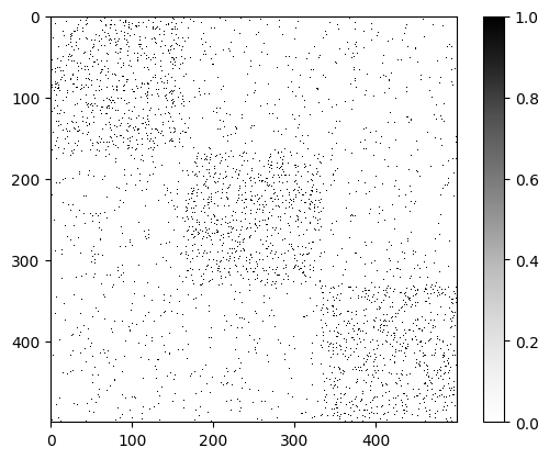
It is now more evident that the input data has indeed three communities, which matches the results given by the cross validation.
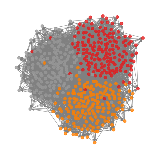
We can now use the inferred parameters to plot the graph together with the communities.
import numpy as np

# Get the community with the highest probability for each node
umax = np.argmax(u, 1)

# Draw the graph using the spring layout
plt.figure(figsize=(5, 5))
nx.draw(
    A[0],
    pos=pos,
    node_size=50,
    node_color=umax,
    alpha=0.8,
    edge_color="gray",
    with_labels=False,
    cmap=plt.cm.Set1,
)
plt.show()
Anomaly Detection#
As we have seen, the ACD method also provides information about the anomalies. We can use the
inferred parameters pi and mu to build a matrix Q that represents the probability of each
edge being an anomaly. We can then set a threshold to determine which edges are anomalous. We can
decide which threshold to use based on the distribution of values in Q.
from probinet.evaluation.expectation_computation import (
    compute_mean_lambda0,
    calculate_Q_dense,
)

# Calculate the matrix Q
M0 = compute_mean_lambda0(u, v, w)
Q = calculate_Q_dense(graph_data.adjacency_tensor, M0, pi, mu)

# Plot the distribution of values in Q
fig = plt.figure(figsize=(7, 3))
plt.hist(Q[0].flatten(), bins=100)
plt.title("Q distribution")
plt.show()
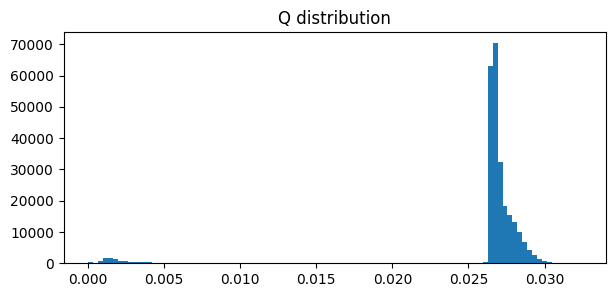
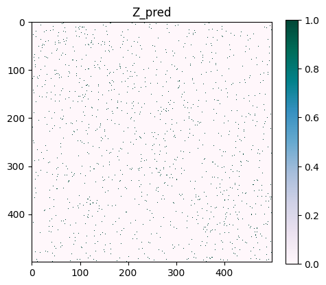
The distribution of values in Q is skewed, with most values close to 0.027. We can concentrate on the most anomalous values by selecting the top 1%.
# Create a mask for the edges
mask_tmp = np.zeros(adjacency_matrix.shape)
mask_tmp[adjacency_matrix.todense() > 0] = 1

# Calculate the threshold for the top 1% most anomalous edges
threshold = np.percentile(Q[0]*mask_tmp, 99)

# Create a copy of Q and set the top 1% most anomalous edges to 1, and the rest to 0
Z_pred = np.copy(Q[0]*mask_tmp)
Z_pred[Z_pred >= threshold] = 1
Z_pred[Z_pred < threshold] = 0

plt.figure(figsize=(5, 5))
cmap = "PuBuGn"
plt.imshow(Z_pred, cmap=cmap, interpolation="none")
plt.colorbar(fraction=0.046)
plt.title("Z_pred")
plt.show()
Summary#
In this notebook, we explored the ACD (Anomaly and Community Detection) model. We began by loading and visualizing the data after importing the necessary libraries. Next, we performed cross-validation by defining both model and cross-validation parameters, using the cross_validation function from the model_selection module. The results were then loaded to identify the optimal number of communities K based on the AUC scores.
With the best K value determined, we proceeded by running the ACD algorithm. For community
detection, we validated the choice of K by plotting the adjacency matrix and visualizing the
graph with the detected communities. For anomaly detection, we computed the matrix Q, which represented the probability of each edge being an anomaly.